In surrogate modelling, to get a uniform coverage of the parameter domain and get as much information about the objective value’s variability per dimension with the least possible input data, we need an adequate design of experiments (DoE), also known as a sampling plan. Such a design is used to determine the inputs with which we run the initial set of simulations that will be used to construct our initial surrogate model(s). Since we are considering a deterministic computer experiment, the DoE does not consider re-sampling for the same input.

Latin Hypercube Sampling

The most popular technique is called Latin Hypercube Sampling (LHS). In this method, each dimensional axis gets divided into a predefined amount of bins equal to the total amount of samples. In each bin, only one sample will be placed. In 2D this means one sample will occupy a row and a column and no other sample can be placed in that row and column.

Although this procedure will result in a so-called ‘stratified’ sampling plan, it is not necessarily optimally ‘space-filling’ or uniform as desired. Therefore the sampling plan is further optimised using some optimality criterium. An effective and popular choice is the maximin criterium, also called the Morris & Mitchell criterium (Citation: Morris & Mitchell, 1995 Morris, M. & Mitchell, T. (1995). Exploratory designs for computational experiments. Journal of Statistical Planning and Inference, 43(3). 381–402. https://doi.org/10.1016/0378-3758(94)00035-T ), in which we select the sampling plan that maximises the minimum (Euclidean) distance between any sampling location. Optimally, we search all possible LHS plans according to this criterion using a divide and conquer method (Citation: Forrester, Sóbester & al., 2008 Forrester, A., Sóbester, A. & Keane, A. (2008). Engineering Design via Surrogate Modelling . John Wiley; Sons, Ltd . https://doi.org/10.1002/9780470770801 ). However, this is computationally expensive and in practice we can search for such a plan iteratively. The Python library pyDOE2 provides the iterative DoE implementation.

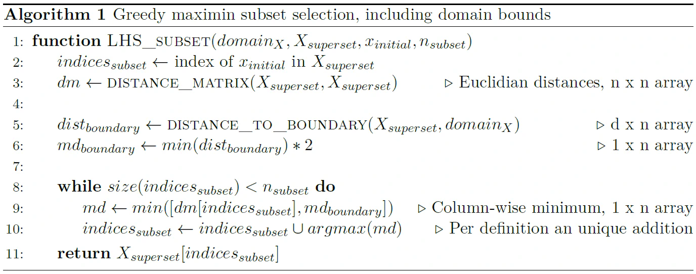
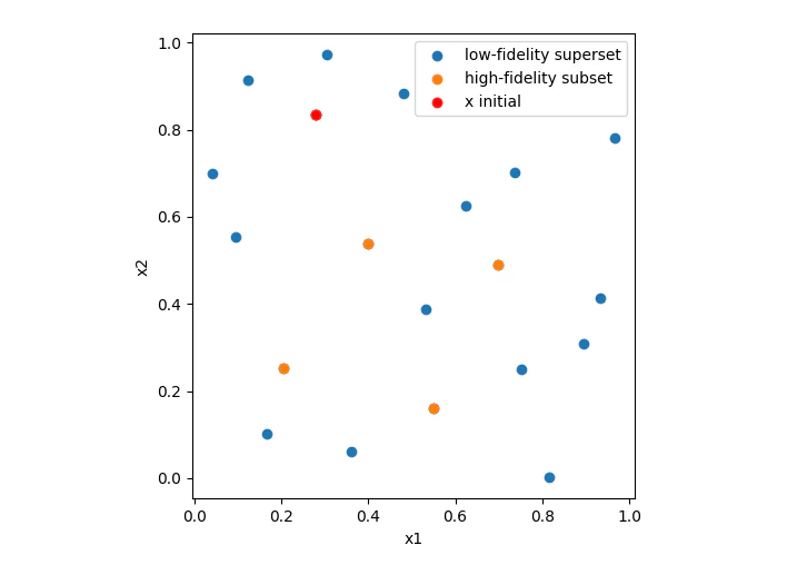
In the multi-fidelity setting, now that we have found an optimised DoE for our lowest fidelity or fidelities, we would like to select a subset of that sampling plan to construct a DoE for the higher fidelity. To generate such an initial high-fidelity DoE, we greedily select points from the already defined lower-fidelity DoE in a similar fashion to Citation: Forrester, Sóbester & al. (2008) Forrester, A., Sóbester, A. & Keane, A. (2008). Engineering Design via Surrogate Modelling . John Wiley; Sons, Ltd . https://doi.org/10.1002/9780470770801 following the maximin principle. However, contrary to (Citation: Forrester, Sóbester & al., 2008 Forrester, A., Sóbester, A. & Keane, A. (2008). Engineering Design via Surrogate Modelling . John Wiley; Sons, Ltd . https://doi.org/10.1002/9780470770801 ), we take the distance to the input domain boundary into account and start with the location of the sample with the current best lower fidelity objective function. The total greedy selection algorithm is expressed in the pseudocode of Algorithm 1 below. An example result of the combined LHS and subset selection is given by this image.

In line 6 of the algorithm I multiply the distance by a factor of two. This is because the goal is to maximise the minimum distance to a source of information. Objective value information is supplied by two sources for distances between sampled locations. In the distance to the boundary, there is only one source of information. To compensate for this we should therefore divide the values of the distance matrix- or equivalently multiply the distances to the boundary by a factor of two. As an analogue for those familiarised with CFD, we effectively calculate the distance to a mirrored non-existing ‘ghost point’.

Size of the initial DoE

The size of the initial Design of Experiments is of large importance to the accuracy of the initial surrogate model and the cost of (initial) sampling. Too many samples may turn out to be overly costly. On the other hand, too few samples provide us with an inaccurate initial surrogate model, causing a less effective optimisation stage. According to e.g. Citation: Toal (2015) Toal, D. (2015). Some considerations regarding the use of multi-fidelity Kriging in the construction of surrogate models. Structural and Multidisciplinary Optimization, 51(6). 1223–1245. https://doi.org/10.1007/s00158-014-1209-5 ; Citation: Forrester, Sóbester & al. (2008) Forrester, A., Sóbester, A. & Keane, A. (2008). Engineering Design via Surrogate Modelling . John Wiley; Sons, Ltd . https://doi.org/10.1002/9780470770801 , $N = 10 \cdot d$ is an effective rule of thumb.

Furthermore, Citation: Picheny, Wagner & al. (2013) Picheny, V., Wagner, T. & Ginsbourger, D. (2013). A benchmark of kriging-based infill criteria for noisy optimization. Structural and Multidisciplinary Optimization, 48(3). 607–626. https://doi.org/10.1007/s00158-013-0919-4 states that the size of the initial DoE in noisy optimisation is not critical to the performance of that optimisation, meaning that the effect of having more initial samples is counterbalanced by having to do fewer sequential sampling steps and vice versa.

Bibliography