Introduction

When I first started learning Python somewhere in 2013, I tried my hand at visualizing the Mandelbrot fractal: A simple mathematic formula with inifinite complexity, that can create the most wondrous of images. Somewhere past year, I decided to pick up on this toy-project again.

At first just for fun; but later I set the goal to create my own ‘benchmark’ of the difference in performance and coding-experience between Python and C++ while we are at it, actively programming in both on a day-to-day basis (in time I might add javascript/typescript to this experiment too).

You (very) roughly encounter the following opinions:

• Execution time: “Python is slow, C++ is fast”
• Developing experience:
  • “Python is easy and fast to develop, C++ is hard and slow”
  • “Interpreted Python is bug-prone; typed and compiled C++ is the way”

Ofcourse, we could continue this and get stuck in a “Interpreted vs Compiled” discussion; and I won’t: Compiled will typically win when purely considering performance, while the developing experience is as heavily opiniated as it is dependent on the use-case and experience of the developer. In the end, the answer always remains: ‘It depends’. My personal goal here is just to first-hand create a direct comparison on these topics, and between these languages.

Performance-wise: It is very easy to write a slow Python program, while a smart (C++) compiler will provide you with many of-the-shelf optimisations (altough it also still is pretty easy to write a slow C++ program). However, I have always developed my Python codes with performance in mind, and when people say that Python is slow: Often it really is the implementation that is (really) slow.

Actual bad implementations aside, Python and it’s ecosystem is king in interfacing with other languages and using their strengths, while retaining it’s own. Think Numpy, Pandas (or Polars) and Numba (which even compiles your Python/Numpy code to execute as C/C++), among many others. Powerful tools harnessing the power of C/C++/Rust, in these cases, with the interpreted scripting and fast prototyping convenience of Python.

This about concludes my motivation of this personal project, and why I let it grow to something worth writing about. Without further ado: let’s introduce the Mandelbrot set.

The Mandelbrot Set

The mandelbrot set’s equation is simple:

$$\begin{equation}\label{eqn:mandelbrot} z_{n+1} = z_n^2 + c, \quad z_0 = 0, \end{equation}$$

Here, $c$ is an imaginary number, and so will be $z$.

The set of numbers $c$ for which this series does not diverge to infinity as $n \rightarrow \infty$ is called the Mandelbrot set. We can do as many iterations as we like, $z_n$ will always be bounded if $c$ is in the set.

To create images, the real and imaginary axis of $c$ is mapped to a pixel x-y location. Pixels correspond with values of $c$ that are in the set are typically colored black, found ‘on the inside’ of the characteristic shape.

Ploting the Mandelbrot equation

In practice, to create our colorfull images, we will calculate $\cref{eqn:mandelbrot}{1}$ $N$ times. However, if we do this naïvely we arrive at a binary answer (“in the set” or “not in the set”), and create black and white images. Not very appealing.

Instead, a mathematical threshold exists after which we are certain the series will diverge. Using this, we might conclude at any iteration that $\cref{eqn:mandelbrot}{1}$ will diverge for this value of $c$, and stop iterating. This measure of how fast $c$ diverges can be all integer values in $[0, N]$. Apply this to a colormap, and we have a colored image! This threshold is called the escape radius.

Escape radius

The escape radius is called as such because it is related to the magnitude of $z_n$, which in the imaginary plane is a radius. After this radius, your equation will escape, like a photon passes the event horizon of a black hole.

The escape radius for the Mandelbrot Set’s equation $\cref{eqn:mandelbrot}{1}$ is 2. This might seems as a random number but makes sense if you see the math. A clear proof, that actually shows where the ‘2’ comes from, and not just shows it works for that number, is given on this website, which I will quote here verbatim:

    The sequence generated by f(z) = z^2 + c beginning with 0 begins

    0, c, c^2 + c, ...

    Call these terms z0, z1, z2, ... .

    In fact this sequence will be unbounded if any of its terms 
    has magnitude larger than 2. 

    The main idea is that if the magnitude |z| is bigger than both 
    2 and the magnitude |c|, then |f(z)|/|z| > |z| - 1 > 1, so that
    by induction the sequence of magnitudes will grow geometrically. 

    To establish the inequality, note that 

    |f(z)|/|z| = |z^2 + c|/|z|
                >= (|z|^2-|c|)/|z|          [ triangle inequality ]
                = |z| - (|c|/|z|) 
                > |z| - 1                  [ |z| > |c| ]
                > 1                        [ |z| > 2 ]

    If  |c| <= 2 and  |zn| > 2 then certainly 
    z = zn satisfies these hypotheses, so the sequence is 
    unbounded.  

    If |c| > 2 then |c^2+c| >= |c|^2 - |c| = |c|(|c|-1) > |c| > 2
    so that z=z2 satisfies the hypotheses of the argument above.

So, if $|z_n|\geq 2$ then we are certain that $c$ is not in the set, and we stop iterating. Note that 2 is a required minimum, if you want you can pick a higher number.

We normally calculate $|z_n|$ and compare as: $$\begin{equation} |z_n| = \sqrt{x^2+y^2} \geq 2 \end{equation}$$ However, since we want to avoid taking the computationally heavy square root, we instead typically do: $$\begin{equation} |z_n|^2 = \left(\sqrt{x^2+y^2}\right)^2 = x^2+y^2 \geq 2^2 = 4 \end{equation}$$ Since this number 4 is not strictly a radius anymore, it is often referred to as the ‘bailout’.

(Smooth) Coloring

The simplest way to color the Mandelbrot equation is to take the iteration count, apply them to a colormap (or anything that maps a scalar to a color), do this for every pixel linked to a $c$, et voilá. Ideally, take a continous and cyclic colormap (starts and ends with the same color), and also make the iteration count loop (i.e. n % 255).

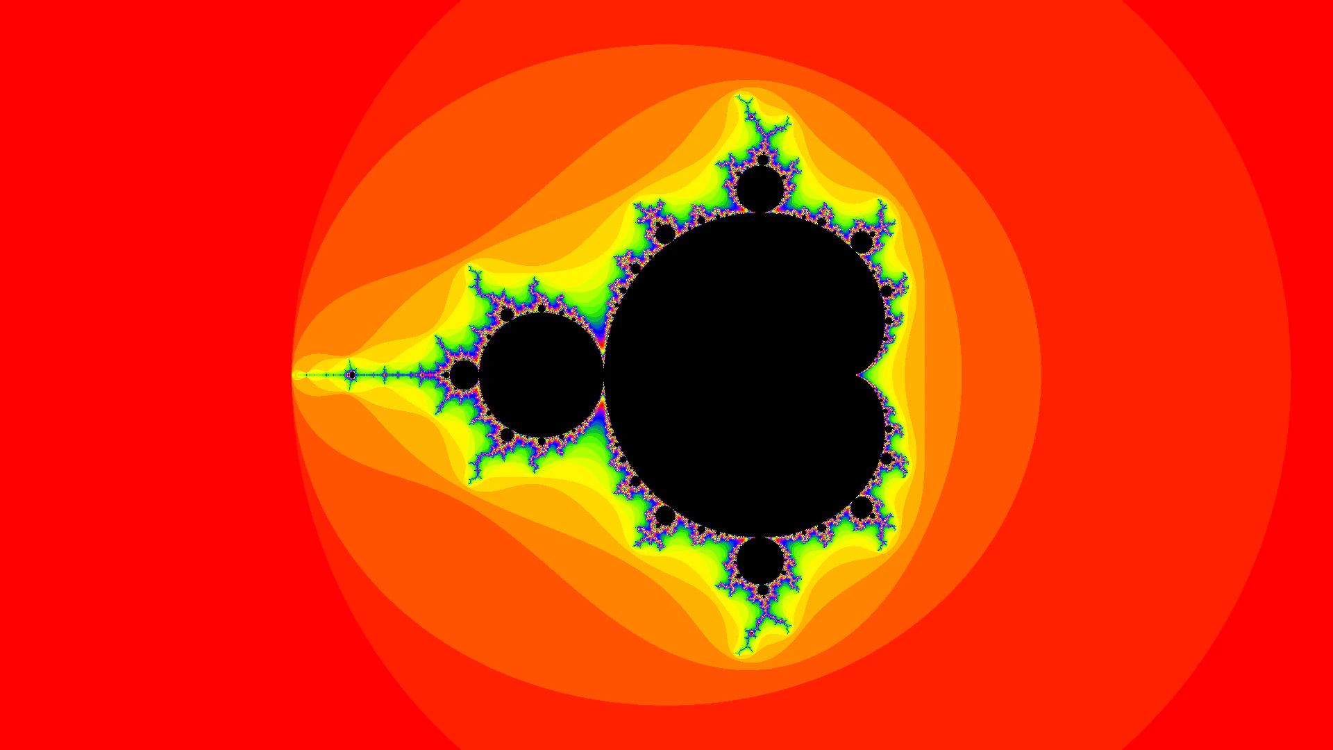
However, since each iteration number $n$ is an integer, this will result in ‘bands’ of color, see Figure 1a.

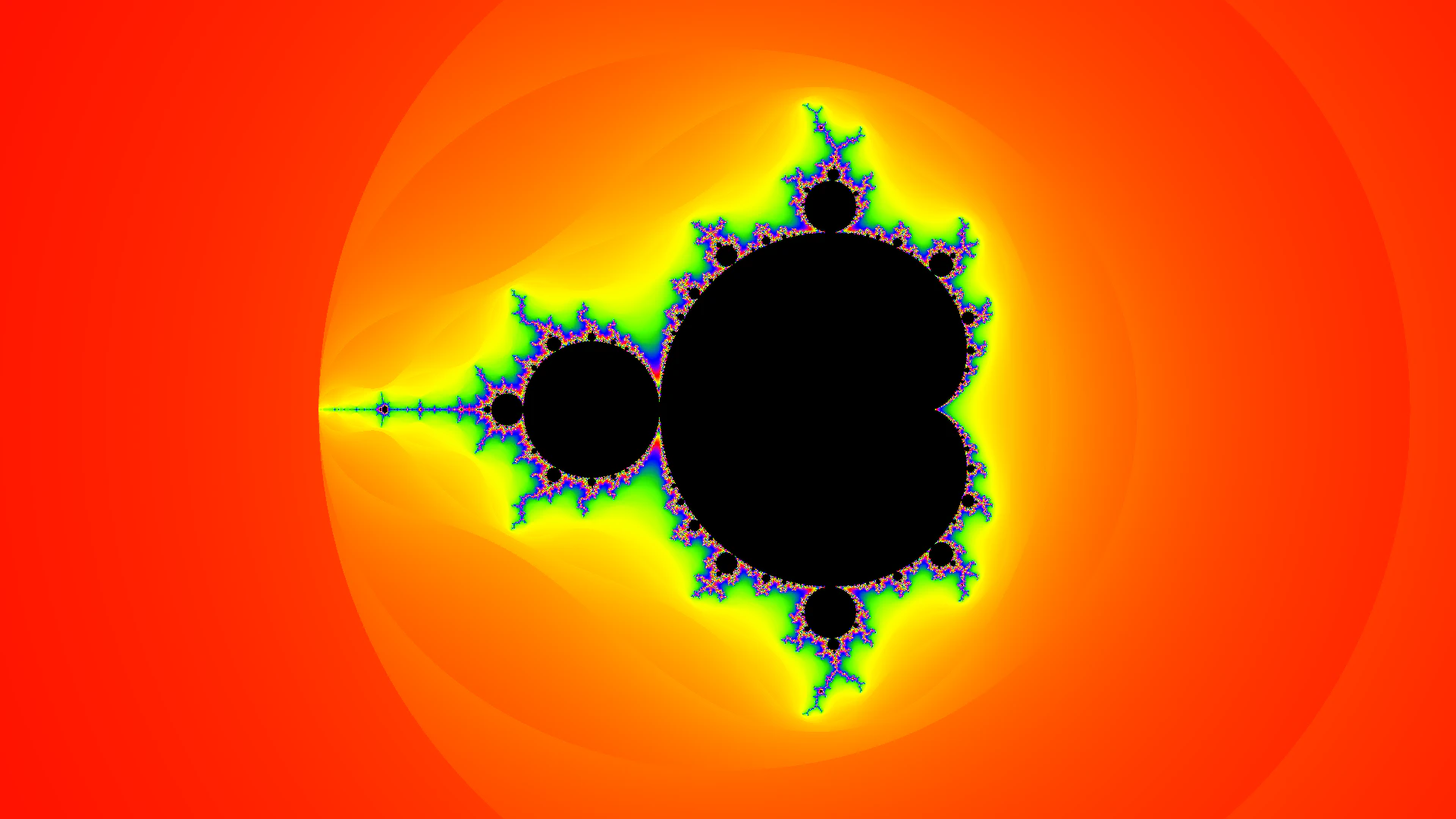
Instead, we would like to transform our iteration count to a float representation, using a measure of how close we were to the escape radius when we exceeded it. Mathematicians came up with the following formula:

$$\begin{equation}\label{eqn:nfrac} n_{frac} = n + 1 - \frac{\ln\ln|z|}{\ln 2} \end{equation}$$

When programming this, we can simplify this a bit for efficiency:

1
2
3

log_zn = np.log(x2 + y2) / 2    # x2, y2: squared real, imaginary parts of z_n
nu = np.log(log_zn) / np.log(2) # precompute ln(2) too!
n_frac = n + 1 - nu

log_zn can be calculated as it is because the magnitude of an imaginary number simply follows Pythagoras’ theorem, after which we apply the power rule of logarithms: $$\begin{equation} \ln|z| = \ln{\left(\sqrt{x^2+y^2}\right)} = \ln{\left(\left(x^2+y^2\right)^\frac{1}{2}\right)} = \frac{\ln{(x^2+y^2)}}{2} \end{equation}$$

Unfortunately, I am not enough of a mathematician to understand, let alone explain the math behind this equation, which actually turns out to be complicated. The DIY linearized bounds argument of this blogpost, might give a first feeling on the subject. However, the ‘simplified explanation’ on this webpage provides insight into the actual formula:

The following simplified and very insightful explanation is provided by Earl L. Hinrichs:

    "Ignoring the +C in the usual formula, the orbit point grows by Z := Z^2. 
    So we have the progression Z, Z^2, Z^4, Z^8, Z^16, etc. 
    Iteration counting amounts to assigning an integer to these values. 
    Ignoring a multiplier, the log of this sequence is: 1, 2, 4, 8, 16. 
    The log-log is 0, 1, 2, 3, 4 which matches the integer value from the iteration counting. 
    So the appropriate generalization of the discrete iteration counting to a continuous function 
    would be the double log."

This simplified explanation also provides a simple insight into why a division by the 
logarithm of the power is required: consider iterating Z := Z^3. 
The log of the sequence yields 1, 3, 9, 27, 81, 243 ... and the double-log yields 
0, log(3), 2log(3), 3log(3), 4log(3), ....

As a result, Figure 1 shows the Mandelbrot set plotted using unsmoothed integer (a) and smoothed fractional coloring (b). The colormap is Matplotlib’s ‘prism’, which is a bit too intense to be pretty, but illustrative.