What is surrogate modelling?

Surrogate modelling creates a computer model that can cheaply replace an expensive or otherwise hard to retrieve function. To intuïtively understand what surrogate modelling is, I would like to use a example.

In the following, let’s consider a problem where we want to find an object shape (a design) that minimises the (de-)acceleration when this object is dropped onto a flat water surface. This is an optimisation process, where we want to find the best design, and prefer to do that as efficiently possible.

We can systematically change (some aspect of) the design and can say something about the quality of that design by the means of simulation tools or other so-called objective functions (in this case the acceleration).

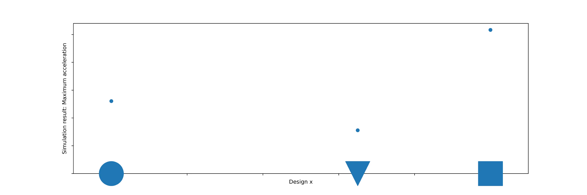
The x-axis shows the design that follows from the systematic design variations, and the y-axis express the (de-)acceleration.

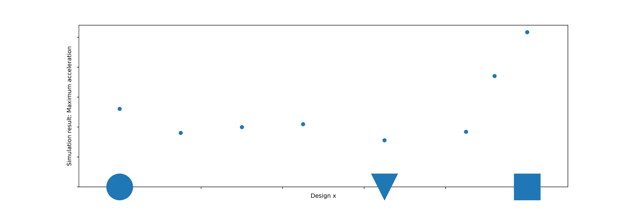
In Figure 1, we have found the accelerations for some designs. Although the triangular design seems to be the best for now, we cannot be very certain about that observation, so let’s try some more designs:

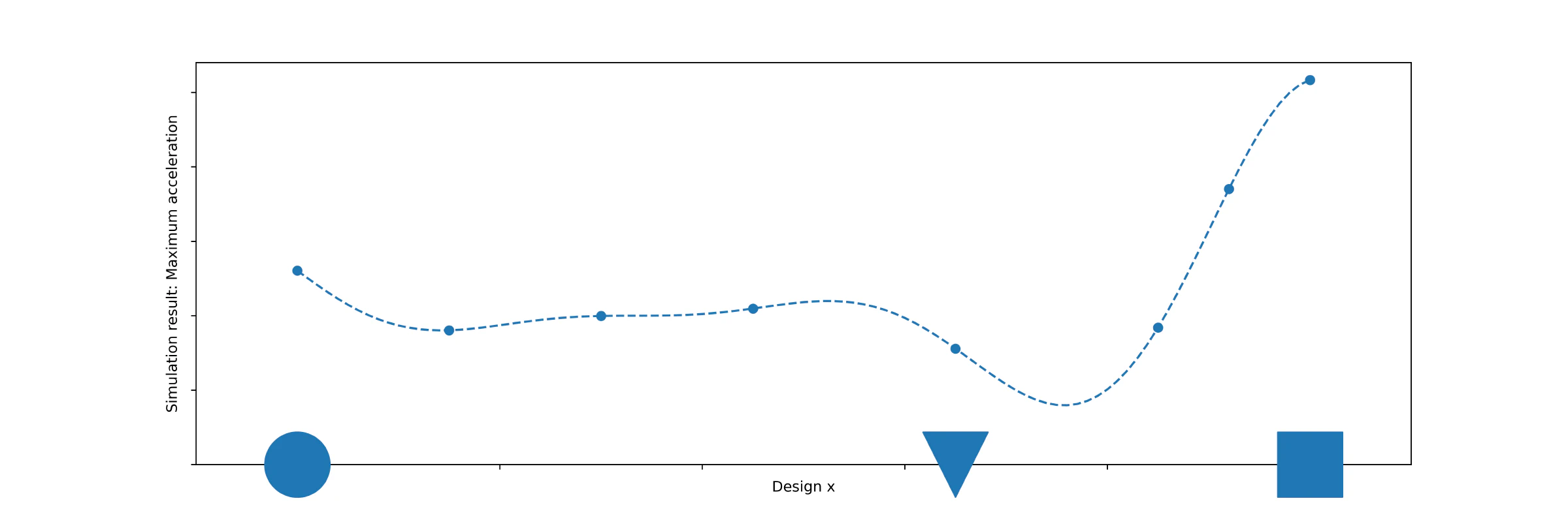
Now that we have tried more designs, we (as humans) might have some intuïtion as to what design is a good candidate to try next. However, computers do not have this intuïtion, and that is where a surrogate model comes in. This is a model, fitted to the data, that replaces the “true” objective function with a cheap-to-evaluate alternative. This surrogate model is given by the blue dashed line in Figure 3.

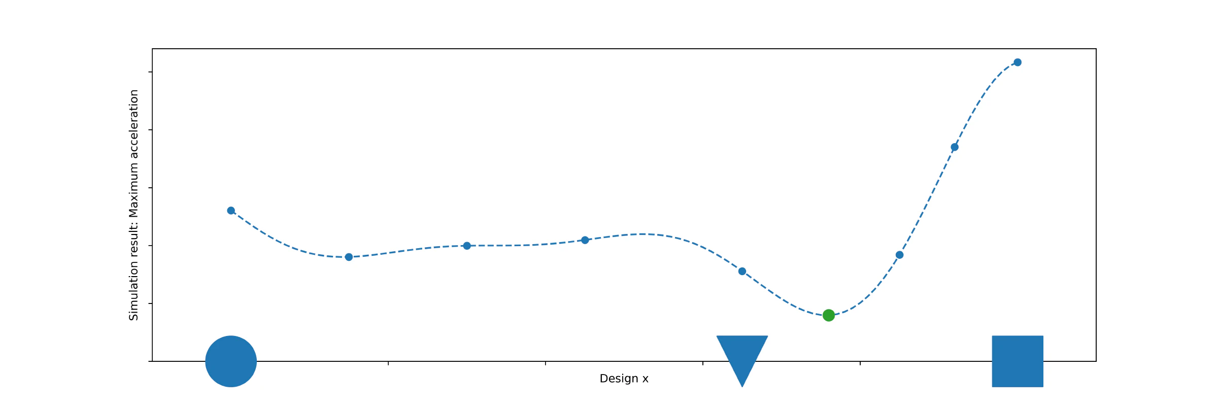
With this surrogate model, the computer also has some ‘intuïtion’ as to what might be an interesting candidate for the best design. Maybe try the design corresponding to the green point in Figure 4?

What can we use surrogate modelling for?

Now that the computer has some data-informed idea about how the true objective function looks like, we can use this cheap predictor of the truth (the surrogate model) for various purposes. With this predictive capability, surrogate models are used for the following goals:

• Speeding up optimisation: Whenever the objective function is computationally expensive to evaluate (such as is the case with CFD or FEM), the surrogate provides a very cheap estimate. This vastly reduces the amount of expensive objective function evaluations, compared to for instance brute-forcing an optimisation.
• Multi-Objective Optimisation: Efficiently search for a Pareto-optimal set by creating a surrogate model per design objective.
• Design exploration: Inherent to the capabilities of surrogate models needed for optimisation, surrogate models can be used for general exploration of the design space.
• Sensitivity Analysis: What parameters best explain the variability of the objective function?

There are a lot of techniques to create surrogate models. Linguistically, the definition of a surrogate model stretches as far as the large Artificial Intelligence/ Machine Learning models we know nowadays: it ‘replaces’ the truth or real-world data. However, you would not see the term ‘surrogate model’ used in such a context, and my own definition is ‘any such model that has a physically interpretable representation’. For instance, more classic and interpretable machine learning methods such as Support Vector Machines (SVMs) are considered surrogate models, while Large Language Models (LLMs) are not.

However, most surrogate models are only capable of producing a prediction. Surrogate modelling really becomes interesting to engineering or other areas that require (mathmatically) provable accuracy when we cannot just predict but also estimate the corresponding model uncertanties (how certain are we about the model prediction at location $x$?). This is where Gaussian Process Regression(GPR) / Kriging comes in.

Now that we have access to the estimated model variances, we can use the Kriging surrogate model for:

• Bayesian Optimisation: Optimisation not just based on the model prediction (the expectation), but taking the model’s whole posterior distribution into account.
• Uncertainty Quantification (UQ): What is the probability distribution of the objective value when the inputs are random variables? This could for instance crudely be done by Monte Carlo simulations, enabled by the surrogate’s cheap predictions.
• Optimisation Under Uncertainty (OUU) & Reliability Based Optimisation (RBO): Two closely related optimisation paradigms that take the input uncertainty into account during optimisation. OUU focuses on finding robust solutions that perform well across various uncertain scenarios, while RBO focuses on optimising systems to meet specified reliability or safety criteria, ensuring low probabilities of failure. Uncertainty Quantification is the foundation of both.

Technically UQ, OUU and RBO do not require the model uncertainty estimates of GPR/Kriging. For instance, Radial Basis Functions (RBF) could also be used as the surrogate model. However, considering the goals of UQ, OUU and RBO they are typically combined with GPR/Kriging.